How To Make Excel Find Duplicates in Columns or Rows

Tutorial Teaching How to Identify Duplicates in Excel

If you use Microsoft Excel, you need to learn how to identify duplicates in columns or rows of data. In this tutorial, I'll show you a few simple tips and tricks that you may find very cool and practical.

Watch this video tutorial to get started…

1. Excel's Remove-Duplicates Tool

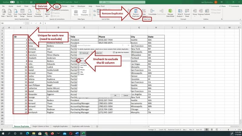
If you want to eliminate duplicates from your dataset, take advantage of the built-in “Remove Duplicates” command on the ribbon:

1. Click anywhere in your data (or select the entire data set)
2. Click on the Data tab on the ribbon
3. Click on the Remove Duplicates button (it's on the Data Tools group of commands)
4. In the dialogue box that pops up, select the columns that identify duplicate rows
5. Click, OK

The screenshot image below shows you the steps:

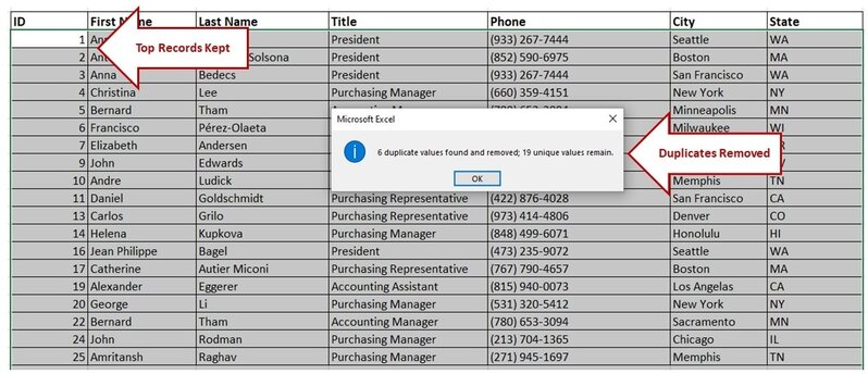
After you click OK… Excel removes duplicates and shows you a confirmation dialogue box, telling you how many duplicates it found and removed:

Important Points to Remember:

• Excel keeps one duplicate and deletes the rest. The question is, which one of them does it keep?

The answer is simple: The topmost duplicate!

Excel sifts through data line by line starting at the top and moving down the dataset, and if it discovers a row with the exact data that it has already “seen,” it deletes it.

• It's very important to select the right combination of columns that define the duplicates. If you include a column with unique values for each record, there will be no duplicates. If you forget to check-mark a column that should be included, you'll lose data.

Now you may stop and think… it's all great stuff, but what if I don't want to delete the duplicates, I just want to find them on the screen?

Great question! It brings me to the second option…

2. Highlight Duplicates With Conditional Formatting

Excel conditional formatting is a great way to identify duplicates. The easiest example is when you are comparing values in individual cells in a range.

Here's how to do it:

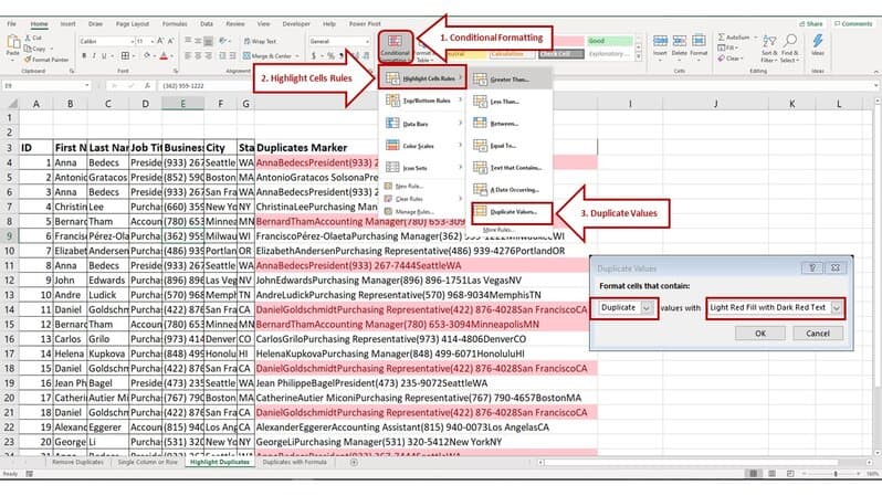
1. Select the range with suspected duplicates
2. Go to Home>Conditional Formatting>Highlight Cells Rules>Duplicate Values
3. Select the style you want to use for highlighting cells with duplicates and click OK.

You can follow the numbered instructions on the picture below:

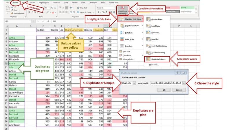
NOTE: You can use this tool not only to highlight duplicates but also to highlight unique values. (See step 5 in the picture above.)

I know… this technique can make Excel find duplicates in a column, and display them, it does not solve the real problem. Like… what if you want to teach Excel to find duplicates in two columns or three or more? Kind of like the Remove-Duplicates command that uses multiple columns to find duplicates but without deleting them.

Here's one more tip…

3. Mark Duplicates With a Formula and Conditional Formatting

The next technique uses three main steps…

• First, create a calculated column;
• Second, apply conditional formatting to that column;
• Third, hide the value in that column. Or… in more detail:

Step 1: Create a New Column and Fill it With a Concatenation Formula

In this step, insert a new column in your dataset and create a formula that combines values from all the columns you want to use for identifying duplicate records. This operation is called concatenation and you can do it using either the CONCATENATE or CONCAT function (you can also use a formula based on the & ampersand or concatenation operator).

Here's a screen shot that shows the exact formulas:

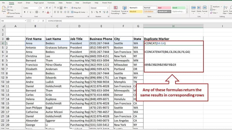
NOTE: The CONCAT function shown in cell H4 is the easiest to use in this case. It's also a newer function. If you can't find it, use one of the other two options, the older CONCATENATE function or the & (ampersand operator) formula.

Step 2: Apply Conditional Formatting to Highlight Duplicates

These steps are already familiar, and a picture is worth a thousand words, so here it goes…

Step 3: Apply Custom Number Format to Hide Concatenated Values

Now… you don't want the long concatenated strings of combined columns displayed in the new duplicates-marker column. Why not hide them with custom number formatting code. The code is ;;; (three semicolons).

Here's how to apply the custom format:

1. Select the Duplicate Marker column.
2. Open the Format-cells dialogue box. You can use Ctrl+1 shortcut, or click on the number-format dialog box launcher button.
3. Click on the Number tab and then on Custom.
4. In the formatting-code box Type ;;; (three semicolons).
5. Click OK to apply your changes.

Again, the picture below shows you step-by-step instructions…

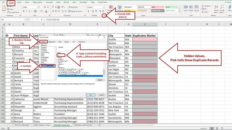
The concatenated text strings in column H are now hidden, the conditional format shows you rows containing duplicate records. Your spreadsheet looks much cleaner and more impressive. Life is good!

Well… it gets even better so keep reading.

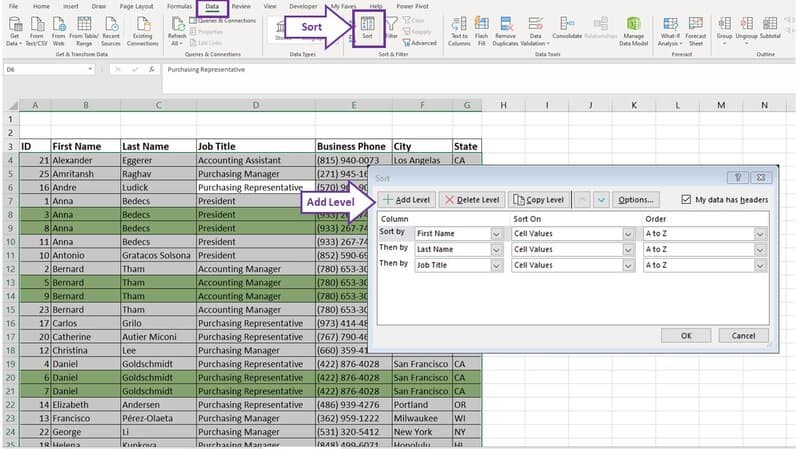
4. Compare Entire Rows by CONCAT

This method is like the previous one, but it allows you to highlight the entire duplicate rows. There is one caveat, however. You must sort the data in a way that groups the duplicate records.

Here's how this technique works:

1. Create a formula that will return TRUE if all the cell values in the current row are identical to those in the row above and FALSE.
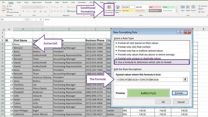
2. Apply a formula-based conditional formatting rule (based on that formula) to your data set.
3. Sort your data to group the duplicates.

Here you are the illustrations with step-by-step instructions:

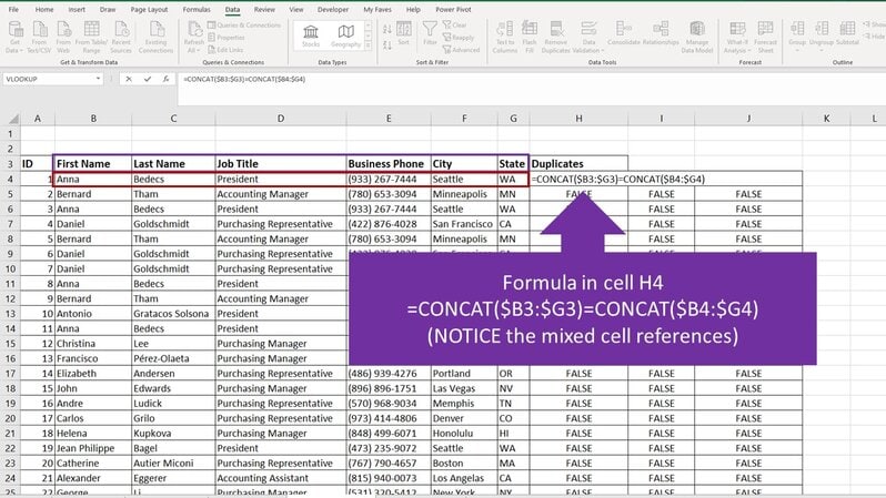
NOTE: The formula must return TRUE if the current row is identical to the one above and FALSE if not. It must also work consistently when copied both vertically and horizontally. That's why it's important to be mindful of using the correct cell references.

I filled the formula in columns H, I, and J for testing and as a proof of concept. It is not strictly necessary. If you are comfortable with conditional formatting, you can easily skip this step.

Now we are ready to sort the dataset and see the duplicate rows.

Notice how I deleted the columns H, I, and J. Like I already mentioned, they were temporary.

You may ask…

Can We Simplify This Solution?

I'm glad you asked because yes, we can… somewhat. Excel Conditional Formatting will work with an Array Formula. Which means you can compare the current row with the row above without having to CONCAT them. Here's how…

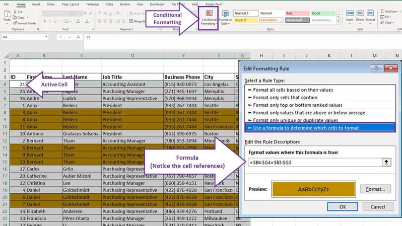
Notice how this formula compares the current row (row 4) to the row above it (row 3). This is an Array Formula. To enter a formula like that in a spreadsheet, you would need to hold Control and Shirt keys and then press enter. In a conditional formatting rule it just works like any other formula that returns a TRUE or a FALSE result.

Isn't conditional formatting great? I advise all my students to learn how to use it.

IMPORTANT: One more time… this technique displays duplicates correctly only when you sort the data properly. I can't emphasize it enough.

Now…

What if you want to keep the entire data set with duplicates and have a list of unique rows at the same time?

Well… in that case you can…

5. Use Excel's UNIQUE Function to Dynamically Extract Unique Rows

If you use a newer version of Excel, you can use the UNIQUE function to identify and extract unique records in your data set. Which is a great technique, because it is dynamic.

Here's how to pull it off…

It's a robust approach to make an Excel table out of your data range first. So, here are the steps:

1. Click in your data set and insert a Table (Insert>Table)
2. In a cell outside the table type the UNIQUE-function formula and press Enter

The UNIQUE function will spill the data into the neighboring cells, so make sure you have plenty of breathing space for that.

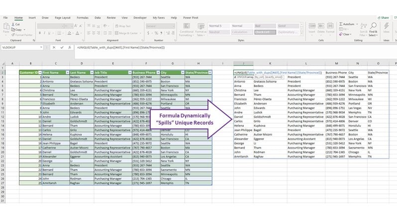
The following figure shows you how and where to create the formula. Note how I left out the Customer ID column from the formula. Otherwise the formula returns all the records because all of them will be unique.

NOTE: Do not type the arguments for this formula. Just type =UNIQUE( and then select the range. In my example, I selected all the columns inside the table except column B with the Customer ID.

You can see the calculation results of the UNIQUE function on the next picture. Notice how this formula spills results into the adjacent cells down and to the right of the cell J2…

NOTE: When you take advantage of this technique, the list of unique records is dynamic. If you add or remove records to the table, the results will change. That is the primary reason to use an Excel table instead of a regular range. The table expands when you add more data to it and it automatically adjusts the function argument for the UNIQUE formula.

It's allows you to keep the duplicates and remove them at the same time. What a nifty way to kill two birds with one stone, isn't it?

Cool… eh?